How to Convert PID Values to Pole Zero Gain Calculator

This calculator converts PID parameters into Pole, Zeros, and Gain. Many people are comfortable tuning feedback loops using PID controllers, but more complex controllers are often specified with s-domain formulas using poles, zeros, and gain. You can use this calculator to bridge the gap between the two tuning methods and hopefully gain insight into how the two approaches relate to each other. This calculator used dB for the gain of the system, so if you want to specify your gain as the signal amplitude out vs. signal amplitude in, you should use the dB Volts Decibel Calculator.

Enter your PID gain values as K_p, K_i, and K_d by adjusting the sliders or manually entering them. You can use the up and down arrows on your keyboard to increment and decrement the values by a minimal amount.

The PID Transfer Function:

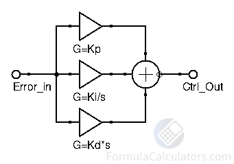
PID Controllers are the sum of a proportional gain (K_p), integral gain (K_i), and derivative gain (K_d). The input to the proportional, integral, and derivative gains is the error between the desired setpoint and the output of the system you want to control. The summed output of the proportional, integral, and derivative are fed into the input of the system you want to control. This configuration creates the full PID feedback loop.

The following transfer function formulas belong to the PID controller itself and don’t include the system you want to control or the error input. The transfer function is shown in the s-domain format, using both its parallel and standard pole, zero, and gain forms. You’ll notice that the PID Controller has a quadratic function in the numerator of its transfer function. This is because some combinations of PID values can create a pair of complex zeros.

PID Controller Transfer Function: 
   
   Again, in standard form.
   
   where:
       • K_p = Proportional Gain
       • K_i = Integral Gain
       • K_d = Derivative Gain
       • s = σ+jω = Laplace Domain Complex Frequency

How to Calculate the Pole, Zeros, and Gain:

You may be looking at the above s-domain formulas and thinking to yourself, “Okay, so how do I get the pole, zeros, and gain from this formula?” If you’re not familiar with Laplace Transforms and dealing with the s-domain, don’t worry. We will review the necessary steps to arrive at the answers and even do a few example problems from easy to somewhat tricky problems. For all examples, we will follow the same three necessary steps.

1.) Substitute the PID settings into the formula, and simplify with algebra.
2.) Factor out your Gain value and convert it to dB.
3.) Find the roots of the numerator and denominator. Then use them to calculate the pole and zero frequencies.

Example #1: Proportional Only

In this example, we have a proportional only PID with the settings:
K_p=2, K_i=0, and K_d=0

Step 1.) Substitute PID settings into the formula.

We’ll do a little algebra simplification here.

$\fn_jvn \small \frac{K_{d}s^{2}+K_{p}s+K_{d}}{s}=\frac{0s^{2}+2s+0}{s}=\frac{2s}{s}=2$

In this case, it simplifies to just the number two! There are no s variables left.

Step 2.) Factor out the Gain, and convert to dB.

For this problem, it’s only a gain of 2, so we need to convert it to dB.

$\fn_jvn \small dB=20log(G)=20log(2)\approx6dB$

So the Gain in dB is 6dB.

Step 3.) Find the roots of the numerator and denominator to solve poles and zeros.

In this case, there are none. Because of this, there are no poles or zeros.

The final answer is 6dB Gain and no poles or zeros.

Example #2: Proportional and Integral

In this example, we have a proportional and integral PID with the settings:
K_p=2, K_i=5, and K_d=0

Step 1.) Substitute PID settings into the formula.

We’ll do a little algebra simplification here.

$\fn_jvn \small \frac{K_{d}s^{2}+K_{p}s+K_{i}}{s}=\frac{0s^{2}+2s+5}{s}=\frac{2s+5}{s}$

This time, we are left with a formula that contains terms of s in the numerator and denominator.

Step 2.) Factor out the Gain, and convert to dB.

The Gain will always be the factor of the highest power of s in our formula’s numerator. The factor next to s is 2, so we will need to pull that factor out in front of our equation.

$\fn_jvn \small \frac{2s+5}{s}=2\frac{\left ( s+\frac{5}{2} \right )}{s}$

You’ll notice how we divided all the terms in the denominator by two so that the s term has a factor of 1. So now we can convert the Gain to dB as before.

$\fn_jvn \small dB=20log(G)=20log(2)\approx 6dB$

Step 3.) Find the roots of the numerator and denominator to solve poles and zeros.

In this case, the numerator and denominator are already factored out. To find the poles, we need to set the denominator to 0 and solve for s. And likewise, set the numerator to 0 and solve for s to find the poles.

Denominator: s = 0
Numerator: 2s+5 = 0

We can see that for the denominator to be zero, s must be zero. So this means there is a pole at 0Hz.

When we solve for s in the numerator, we get s = -5/2. So what do we do with this?

Well, this may be a bit hand-wavy, but the s-domain frequencies are in the units of radians-per-second, and positive frequencies reside on the negative axis. So we need to multiply our result of -5/2 by -1/(2π) to get the Hz frequency answer.

$\fn_jvn \small \frac{-5}{2}\cdot \frac{1}{2\pi }=\frac{5}{4\pi }\approx 0.398Hz$

We found the final answer is 6dB Gain, a Pole at 0Hz, and a Zero at 0.398Hz.

Example #3: Proportional, Integral, and Derivative (easy one)

In this example, we have proportional, integral, and derivative terms in our PID settings:

K_p=8, K_i=5, and K_d=3

Step 1.) Substitute PID settings into the formula.

$\fn_jvn \small \frac{K_{d}s^{2}+K_{p}s+K_{i}}{s}=\frac{3s^{2}+8s+5}{s}$

Unlike the previous examples, we didn’t get much simplification of the formula in this first step.

Step 2.) Factor out the Gain, and convert to dB.

The Gain will always be the factor of the highest power of s in our formula’s numerator. We have a factor of 3*s^2 in our formula, so our Gain is 3. We will need to pull that factor out in front of our equation.

$\fn_jvn \small \frac{3s^{2}+8s+5}{s}=3\frac{\left ( s^{2}+\frac{8}{3}s+\frac{5}{3} \right )}{s}$

Now we convert the Gain of 3 into dB.

$\fn_jvn \small dB=20log(G)=20log(3)\approx 9.542dB$

Step 3.) Find the roots of the numerator and denominator to solve poles and zeros.

Right away, you should notice that the denominator is just s. As you found last time, that means we have a pole at 0Hz. Let’s evaluate the numerator now without the Gain when it’s set equal to zero.

Numerator: $\fn_jvn \small 3\left ( s^{2}+\frac{8}{3}s+\frac{5}{3} \right )=0$

It looks like we have to factor a quadratic formula to determine what values of s make the numerator equal to zero. There are a few ways to do this. One method that always works is the quadratic formula, so let’s go ahead and use it now.

For equations with the form:
$\fn_jvn \small ax^{2}+bx+c=0$
The quadratic formula is:
$\fn_jvn \small x=\frac{-b\pm \sqrt{b^{2}-4ac}}{2a}$

Substituting the numerator of our transfer function, we can see that we can solve s with:

$\fn_jvn \small s=\frac{-K_{p}\pm \sqrt{K{_{p}}^{2}-4K_{d}K_{i}}}{2K_{d}}$

Substituting our variables, and solving for s, we get:

$\inline \fn_jvn s=\frac{-K_{p}\pm \sqrt{K{_{p}}^{2}-4K_{d}K_{i}}}{2K_{d}}=\frac{-8\pm \sqrt{8^{2}-4\cdot 3\cdot 5}}{2\cdot 3}=\frac{-8\pm \sqrt{64-60}}{6}=\frac{-8\pm 2}{6}$

This gives us two solutions for s:

$\fn_jvn \small s=\frac{-8+2}{6}=\frac{-6}{6}=-1$
and
$\fn_jvn \small \frac{-8-2}{6}=\frac{-10}{6}=\frac{-5}{3}$

Remember, as in previous examples; we need to multiply these results by -1/(2π) to get Hz frequency results. This time we have two results for the frequencies of the zeros of this controller.

$\fn_jvn \small Zero_{1}=-1\cdot \frac{-1}{2\pi }=\frac{1}{2\pi }\approx 0.159Hz$

$\fn_jvn \small Zero_{2}=\frac{-5}{3}\cdot \frac{-1}{2\pi }=\frac{5}{6\pi }\approx 0.265Hz$

As a result, the final answer is 9.542dB Gain, a Pole at 0Hz, the first Zero at 0.159Hz, and a second Zero at 0.265Hz.

Example #4: Proportional, Integral, and Derivative (harder one)

In this example, we have proportional, integral, and derivative terms in our PID settings:

K_p=5, K_i=3, and K_d=4

Step 1.) Substitute PID settings into the formula.

$\fn_jvn \small \frac{K_{d}s^{2}+K_{p}s+K_{i}}{s}=\frac{4s^{2}+5s+3}{s}$

Step 2.) Factor out the Gain, and convert to dB.

The Gain will always be the factor of the highest power of s in our formula’s numerator. We have a factor of 4*s^2 in our formula, so our Gain is 4. We will need to pull that factor out in front of our equation.

$\fn_jvn \small \frac{4s^{2}+5s+3}{s}=\frac{4\left ( s^2+\frac{4}{5}s+\frac{3}{4} \right )}{s}$

Now we convert the Gain of 4 into dB.

$\fn_jvn \small dB=20log(G)=20log(4)\approx 12dB$

Step 3.) Find the roots of the numerator and denominator to solve poles and zeros.

As in the previous example, the s in the denominator means we have a pole at 0Hz. We also have a quadratic in the numerator, and we can proceed to solve for the two zeros using the quadratic formula like last time.

$\fn_jvn \small s=\frac{-K_{p}\pm \sqrt{{K_{p}}^{2}-4K_{d}K_{i}}}{2K_{d}}$

Substituting our variables, and solving for s, we get:

$\inline \fn_jvn s=\frac{-K_{p}\pm \sqrt{{K_{p}}^{2}-4K_{d}K_{i}}}{2K_{d}}=\frac{-5\pm \sqrt{5^{2}-4\cdot 4\cdot 3}}{2\cdot 4}=\frac{-5\pm \sqrt{25-48}}{8}=\frac{-5\pm \sqrt{-23}}{8}$

Did you notice that this time, we have a negative number in the square root? The presence of a negative number under a square root results in an imaginary number. Thus, we will get a pair of complex conjugates for solutions for s.

$\fn_jvn \small s=\frac{-5+\sqrt{-23}}{8}\approx \frac{-5+4.796j}{8}\approx \frac{-5}{8}+0.599j$
and
$\fn_jvn \small s=\frac{-5-\sqrt{-23}}{8}\approx \frac{-5-4796j}{8}\approx \frac{-5}{8}-0.599j$

These solutions show you where the complex zeros are in the s-domain, but typically when dealing with complex conjugate poles or zeros, it’s better to refer to them by their natural frequency and damping ratio.

Step 4.) Calculate the natural frequency and damping ratio

We will cover two ways to get the natural frequency and damping ratio. Both are equally valid, but you may find that you like one better than the other. The first method uses the complex numbers that we solved for the zeros’ locations, and the second method solves them directly from the coefficients in the quadratic s-domain equation.

Solving natural frequency and damping ratio with method #1:

We can calculate the natural frequency and damping factor directly with the following formulas because we have already solved the complex conjugate zeros of the PID. The natural frequency is just the vector length of one of the complex zeros. We can find this by using the Pythagorean theorem on one of the zeros’ real and imaginary parts. The damping factor is equal to the negative real part of the complex zero divided by the natural frequency.

$\fn_jvn \small \omega_{0}=\sqrt{\Re(zero)^{2}+\Im(zero)^{2}}$

$\fn_jvn \small \zeta =\frac{-\Re(zero)}{\omega_{0}}$

where:

$\fn_jvn \small \Re$ = Real part
$\fn_jvn \small \Im$ = Imaginary part
$\fn_jvn \small \omega_{0}$ = Natural frequency (radians per second)
$\fn_jvn \small \zeta$ = Damping ratio

Substituting one of our complex zeros, we get:

$\fn_jvn \small \omega_{0}\approx \sqrt{\left ( \frac{-5}{8} \right )^{2}+0.599^{2}}\approx \sqrt{0.391+0.359}\approx \sqrt{0.75}\approx 0.866$

$\fn_jvn \small \zeta =-\frac{\Re(zero)}{\omega_{0}}\approx -\frac{\frac{-5}{8}}{0.866}\approx 0.722$

Note that the natural frequency variable 𝜔₀ is in radians per second, and we will need to convert it to Hz.

$\fn_jvn \small Hz=\frac{\omega_{0}}{2\pi }$

Substituting our natural frequency in radians per second:

$\fn_jvn \small Hz\approx \frac{0.866}{2\pi }\approx 0.138Hz$

We were able to calculate the natural frequency of 0.138 Hz and the damping ratio of 0.722 from one of our system’s complex zeros.

Solving natural frequency and damping ratio with method #2:

You can calculate the natural frequency and damping ratio directly from the transfer function of a quadratic set of poles or zeros. The natural frequency and damping ratio can be found by evaluating this formula that shows the variables in a quadratic function:

$\fn_jvn \small s^{2}+2\zeta \omega_{0}s+{\omega _{0}}^{2}=0$
where:
$\fn_jvn \small \omega_{0}$ = Natural frequency (radians per second)
$\fn_jvn \small \zeta$ = Damping ratio

If you recall, earlier in step #2 we factored out the Gain in the numerator of the transfer function to get the formula:
$\fn_jvn \small 4\left ( s^{2}+\frac{5}{4}s+\frac{3}{4} \right )$

We can generalize factoring out the Gain of the numerator by rewriting it as follows:
$\fn_jvn \small K_{d}\left ( s^{2}+\frac{K_{p}}{K_{d}}s+\frac{K_{i}}{K_{d}} \right )$

If you compare this formula to the natural frequency and damping factor formula, you’ll notice that if you remove the factor of Kd in front (which does not impact the zeros), they match the same form factor.

$\fn_jvn \small s^{2}+\frac{K_{p}}{K_{d}}s+\frac{K_{i}}{K_{d}}=s^{2}+2\zeta \omega_{0}s+{\omega _{0}}^{2}$

From this, we can see:

$\fn_jvn \small {\omega _{0}}^{2}=\frac{K_{i}}{K_{d}}$
and
$\fn_jvn \small 2\zeta \omega _{0}=\frac{K_{p}}{K_{d}}$

Simplifying, we see:

$\fn_jvn \small \omega _{0}=\sqrt{\frac{K_{i}}{K_{d}}}$
and
$\fn_jvn \small \zeta =\frac{K_{p}}{2K_{d}\sqrt{\frac{K_{i}}{K_{d}}}}$

So we can solve the natural frequency and damping ratio of the complex pair of zeros by substituting our PID values:

K_p=5, K_i=3, and K_d=4

$\fn_jvn \small \omega _{0}=\sqrt{\frac{K_{i}}{K_{d}}}=\sqrt{\frac{3}{4}}\approx 0.866 (rad/sec)$

$\fn_jvn \small \zeta = \frac{k_{p}}{2K_{d}\sqrt{\frac{K_{i}}{K_{d}}}}= \frac{5}{2\cdot 4\sqrt{\frac{3}{4}}}= \frac{5}{8\sqrt{\frac{3}{4}}}\approx 0.722 \zeta$

The natural frequency of 𝜔₀ is in radians per second, but you can convert it into Hz frequency by dividing it by 2*π.

$\fn_jvn \small \frac{\omega _{0}}{2\pi }=\frac{\sqrt{\frac{3}{4}}}{2\pi }\approx 0.138 Hz$

Well, it’s been a long road solving this one. But the final answer is 12dB Gain, a Pole at 0Hz, and a pair of complex conjugate zeros with a natural frequency of 0.138 Hz and a damping ratio of 0.722 ζ.

How to Convert PID Values to Pole Zero Gain Calculator

The PID Transfer Function:

How to Calculate the Pole, Zeros, and Gain:

Example #1: Proportional Only

Step 1.) Substitute PID settings into the formula.

Step 2.) Factor out the Gain, and convert to dB.

Step 3.) Find the roots of the numerator and denominator to solve poles and zeros.

Example #2: Proportional and Integral

Step 1.) Substitute PID settings into the formula.

Step 2.) Factor out the Gain, and convert to dB.

Step 3.) Find the roots of the numerator and denominator to solve poles and zeros.

Example #3: Proportional, Integral, and Derivative (easy one)

Step 1.) Substitute PID settings into the formula.

Step 2.) Factor out the Gain, and convert to dB.

Step 3.) Find the roots of the numerator and denominator to solve poles and zeros.

Example #4: Proportional, Integral, and Derivative (harder one)

Step 1.) Substitute PID settings into the formula.

Step 2.) Factor out the Gain, and convert to dB.

Step 3.) Find the roots of the numerator and denominator to solve poles and zeros.

Step 4.) Calculate the natural frequency and damping ratio

Solving natural frequency and damping ratio with method #1:

Solving natural frequency and damping ratio with method #2:

One comment

Leave a Reply Cancel reply